Introduction to PLS Regression in caliX Suite

What is Partial Least Squares (PLS) Regression?

Near-infrared (NIR) spectra consist of thousands of individual wavelength points. Because NIR light absorption manifests as broad, overlapping vibrational overtones rather than sharp peaks, a single wavelength is rarely sufficient to predict a chemical concentration. We need multivariate statistics, particularly for complex chemical and pharmaceutical applications.

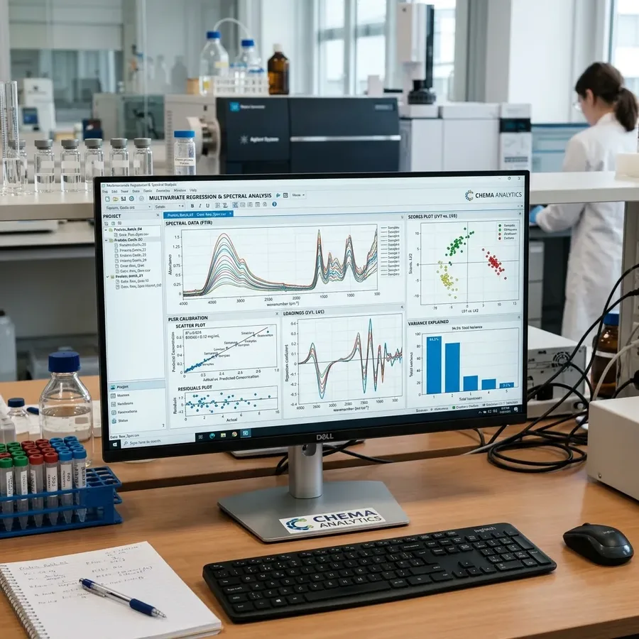
Partial Least Squares (PLS) Regression is the gold standard chemometric algorithm. It reduces the thousands of highly collinear spectral variables into a few orthogonal factors (called Latent Variables (LVs) or principal components) that maximize the covariance between the spectral data and the target laboratory reference concentrations.

Developing a model used to require manual scripting in MATLAB or R. Within the **caliX AutoML Suite** (which constructs highly accurate caliX AutoML models), this workflow is simplified into five clear stages.

---

Step 1: Data Alignment and Import

First, prepare a calibration spreadsheet (CSV or Excel) matching your spectral file names to their wet chemistry laboratory results. caliX supports direct import of raw spectrometer database formats and standard spectroscopic exchange formats like JCAMP-DX.

Once imported, caliX splits your dataset automatically: 75% for Calibration & Cross-Validation (to train the model) and 25% as an Independent Validation Set (kept completely separate to test final predictive performance).

Step 2: Choosing Spectral Preprocessing

Raw NIR light signals contain physical scatter noise caused by particle size variations, sample packing density, or probe distance. Spectral preprocessing mathematically eliminates these physical baselines so the PLS model focuses purely on chemical absorption.

In the caliX pipeline, you can apply and chain standard preprocessing steps:

• Standard Normal Variate (SNV): Centering and scaling each individual spectrum to remove multiplicative scaling and offset variations.
• Multiplicative Scatter Correction (MSC): Regresses each spectrum against the average spectrum to isolate and remove scatter slopes.
• Savitzky-Golay Derivatives (1st or 2nd): Computes local polynomial fits to take derivatives, resolving overlapping bands and removing baseline shifts.

Tip: caliX's AutoML engine will automatically run a grid search over dozens of preprocessing combinations to suggest the optimal sequence for your matrix.

Step 3: Selecting Latent Variables (LVs)

Selecting the correct number of Latent Variables is critical to prevent **overfitting**. If you select too few LVs, your model is underfitted and misses chemical correlations. If you select too many LVs, your model begins fitting random spectral noise, which will fail when scanning new samples.

Look at the Root Mean Square Error of Cross-Validation (RMSECV) curve. Select the number of LVs at the "elbow" of the curve, where the error stops dropping significantly. Adding more components beyond this point only fits noise.

# Sample Model Statistics Output in caliX
---------------------------------------------
Target Parameter: Crude Protein
Preprocessing: SNV + S-G 1st Derivative (15pt)
Selected Latent Variables (LVs): 6

Calibration R—: 0.982
Calibration RMSEC: 0.09%
Cross-Validation RMSECV: 0.11%
Validation RMSEP: 0.12%
Bias: -0.01%
---------------------------------------------
                

Step 4: Independent Validation

To qualify the model for factory deployment, run predictions on the 25% independent test set. The Root Mean Square Error of Prediction (RMSEP) measures the true accuracy you will see when using the sensor inline. A robust model should display an RMSEP that is very close to your cross-validation error (RMSECV).

Step 5: Exporting to ProChem

Once you are satisfied with the model performance, click "Export Model Package". This generates a secure `.caliX` model file. Load this file directly into the ProChem Process Control Software on your production line. ProChem will automatically apply the pre-configured preprocessing steps to inline spectra and predict concentrations in real-time, sending results straight to your plant PLC.

Summary

By combining rigorous PLS regression logic with automated preprocessing optimization, the caliX Suite makes chemometrics accessible to quality control engineers without sacrificing scientific depth. You get reliable, robust models ready to protect your B2B margins on day one.

References

- Martens, H., & Næs, T. (1989). Multivariate Calibration. John Wiley & Sons.
- "Preprocessing Techniques in Near-Infrared Spectroscopy: A Chemometric Guide for Industrial Practitioners," Analytica Chimica Acta, 2022.
- Geladi, P., & Kowalski, B. R. (1986). "Partial Least-Squares Regression: A Tutorial," Analytica Chimica Acta, 185, 1-17.